Most of our clients use Deltek Cobra for Earned Value Management (EVM) analysis of their Primavera P6 schedules. It is, however, possible to perform basic EVM in Primavera P6.
EVM has demonstrated, for well over a 50 years, that it is one of the most effective means available to monitor project cost and schedule performance. EVM quickly reveals poor project planning or the inability to execute a good plan. During project execution and control, EVM provides insight into a projects current cost and schedule status, which helps the project manager balance the triple constraints of cost, schedule, and scope. EVM has many terms to support schedule analysis, some of the more rudimentary variables are available directly in Primavera P6 Professional.
This article demonstrates performing basic EVM in Primavera P6 Professional.
EVM in Primavera P6
Our demonstration project schedule and baseline are displayed in Figure 1. Note that because most EVM programs use much longer reporting cycles, typically a financial or calendar month, this simple example is designed to keep the math easy to follow and note reflect a realistic EVM schedule.
 Figure 1
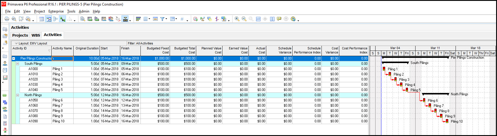
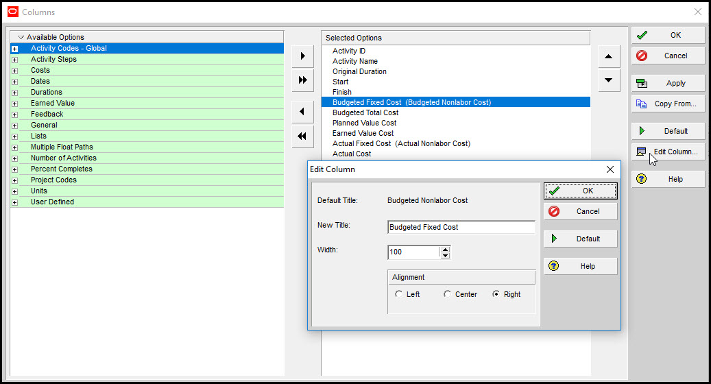
This schedule documents the effort to install pilings for a pier construction project. This project has two deliverables: installation of five south pilings and installation of five north pilings. Each piling is one day duration and has a fixed cost of $100. The fixed cost is stored in the budgeted non-labor cost field. Note in Figure 2 we edit the budgeted non-labor cost column and make a new title, “budgeted fixed cost.
Figure 2
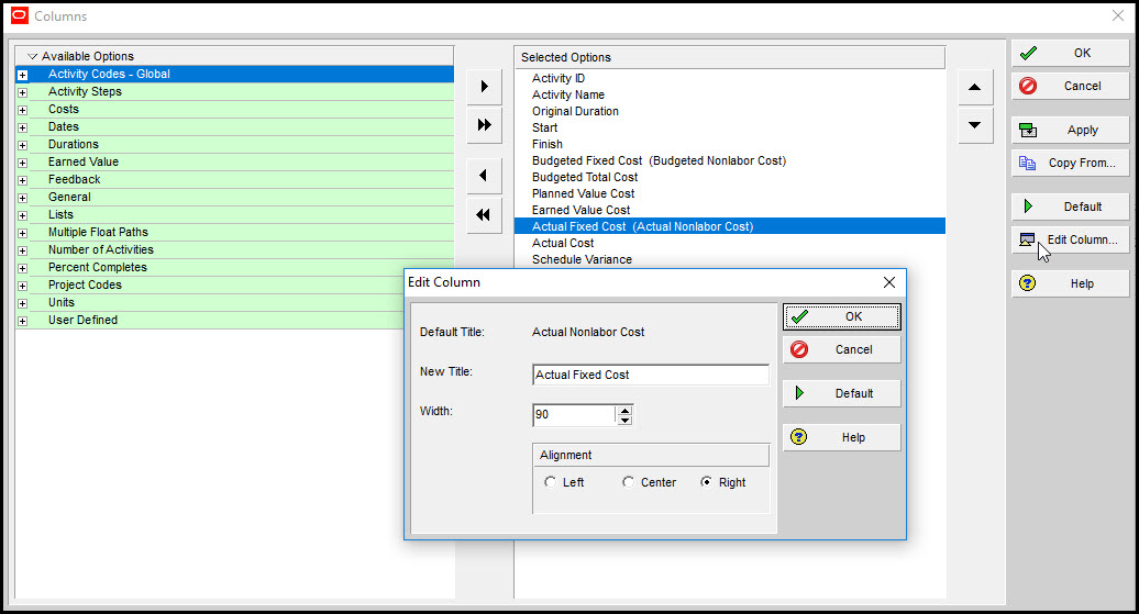
In Figure 3 we also edit the actual non-labor cost column to read “actual fixed cost”.
Figure 3
We proceed and progress the schedule, Figure 4.
Figure 4
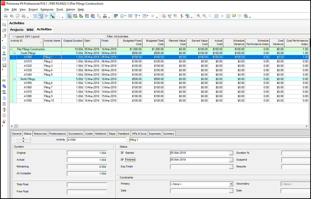
In Figure 4 we enter the started and finished status of piling 1. Note that the planned value fields do not automatically update with this schedule progress. We have to move the data date forward and recalculate the schedule for the planned value fields to populate. In Figure 5 we continue to progress the schedule by specifying the completion of pilings 2 and 3.
Figure 5
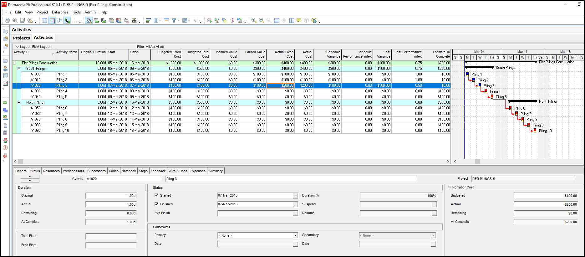
We further enter an actual fixed cost of $200 for piling 3. So piling 3 had $100 cost overrun. Now that our schedule status is entered we can move the data date forward, Figure 6.
Figure 6
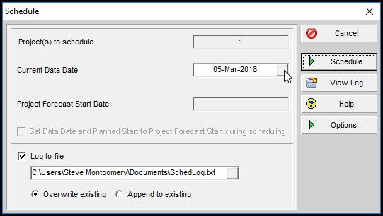
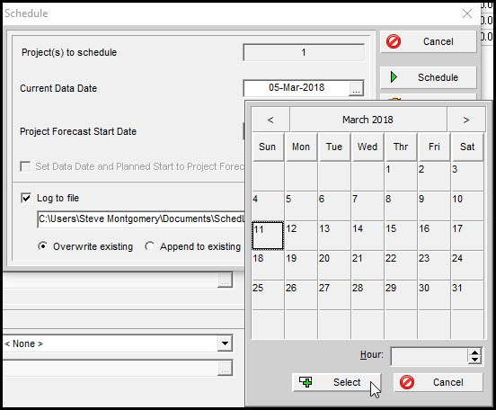
In Figure 6 we select the current data date ellipse button. We move that data date forward one week, Figure 7.
Figure 7
Finally, we recalculate the schedule to arrive at the progressed schedule displayed in Figure 8.
Figure 8
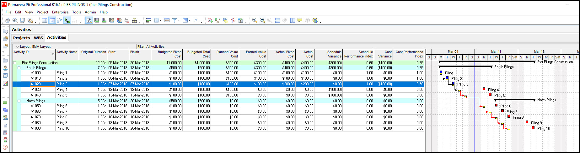
Note that the planned value column is now populated through piling 5. The earned value and actual cost columns are populated through piling 3. Piling 4 and 5 have no progress or associated costs, as per our data date.
EVM Fundamental Parameters
We continue and introduce some of the basic EVM terms exhibited in our schedule, Figure 8. Most earned value parameters are achievable once the planned value (PV), earned value (EV), actual cost (AC), and budget at completion (BAC) values are known. Some of the more fundamental EVM terms are possible with simply the PV, EV, and AC metrics. PV is the value of work planned to be completed, EV is the value of work actually completed, and AC is the funds spent.
EVM Metrics
Let’s look at some of the more rudimentary EVM parameters possible with our three metrics: PV, EV, and AC.
Cost Variance
The cost variance (CV) is computed as follows:
CV = EV-AC
CV compares the value of worked completed, EV, to the AC. The PV, AC, and EV of our piling project are $500, $400, and $300, respectively. Considering only PV and AC it appears that our project is underspent $100. However, when we include EV in our CV formula the CV computes as follows:
CV = $300-$400
CV = -$100
So our project is actually overspent $100. This also demonstrates the EVM paradigm: you compare what you spent to what you accomplished, not what you planned to spend.
Schedule Variance
There are two ways to determine the schedule variance (SV): the dollarized approach and the time units approach. The dollarized SV approach measures from the vertical axis while the time units approach measures from the horizontal axis. The dollarized SV equation is below:
SV$ = EV-PV
The SV$ for our piling project is
SV$ = $300-$500
SV$ = -$200
The negative SV$ value indicates the project is running late. A positive SV$ value would indicate we are ahead of schedule. A value of zero means we are on schedule.
Cost Performance Index
The efficiency of funding spent or the cost performance index (CPI) computes as follows:
CPI = EV/AC
The CPI for our pier piling project is as follows:
CPI = $300/$400
CPI = 0.75
CPI is an important EVM term, because it helps to estimate the final performance requirements to meet funding goals. CPI values less than 1.0 indicate overspending, greater than 1.0 underspending, and 1.0 on budget spending. You can think of CPI as a basic Return On Investment (ROI) calculation: that is to this this CPI tells us we have earned 0.75 cents for every dollar spent.
Schedule Performance Index
The dollarized SPI equation computes as follows:
SPI$ = EV/PV
Our project’s SPI is below:
SPI$ = $300/$500
SPI$ = 0.6
The SPI$ is less than one demonstrates the project is behind schedule. Note that the SPI$ indicates a trend and not an exact value.
Summary
Rudimentary EVM in Primavera P6 Professional is available. Project schedule and cost trend computations are possible with three simple EVM metrics: Planned Value, Earned Value, and Actual Cost. When these three metrics are determined for each project time period one may compute CV, SV$, CPI, and SPI metrics.
However, one must progress the schedule against a baseline to determine the Planned Value, Earned Value, and Actual Cost metrics required for these EVM metric trends. The tool does offer some additional earned value capabilities not discussed in this article. But this should a great starting point for anyone interested in obtaining more thorough metrics from their project schedule.